实验环境
本节使用 NumPy、Matplotlib 和 scikit-image。代码在构建网站时执行,输出图像会直接嵌入静态网页。
生成 Phantom 与正弦图
代码
image = resize(shepp_logan_phantom(), (256, 256), anti_aliasing=True)
theta = np.linspace(0.0, 180.0, max(image.shape), endpoint=False)
sinogram = radon(image, theta=theta, circle=True)

fig, axes = plt.subplots(1, 2, figsize=(10, 4))
axes[0].imshow(image, cmap="gray")
axes[0].set_title("Phantom")
axes[0].axis("off")
axes[1].imshow(
    sinogram,
    cmap="gray",
    aspect="auto",
    extent=(theta.min(), theta.max(), sinogram.shape[0], 0),
)
axes[1].set_title("Sinogram")
axes[1].set_xlabel(r"Projection angle $\theta$ (degree)")
axes[1].set_ylabel(r"Detector coordinate $s$")
plt.tight_layout()
plt.show()
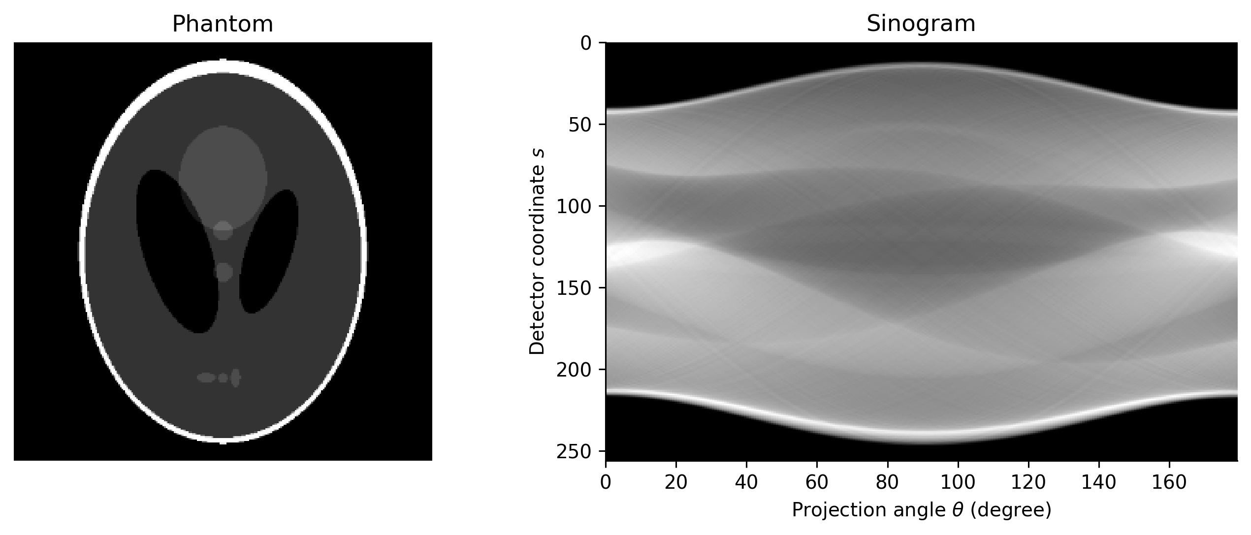
Shepp-Logan Phantom 及其平行束正弦图。
图 1 展示了二维物体与投影空间之间的映射。椭圆边界在正弦图中表现为相互交叠的周期轨迹。
简单反投影与 FBP
代码
backprojection = iradon(
    sinogram,
    theta=theta,
    filter_name=None,
    circle=True,
)
fbp = iradon(
    sinogram,
    theta=theta,
    filter_name="ramp",
    circle=True,
)

fig, axes = plt.subplots(1, 3, figsize=(12, 4))
for ax, data, title in zip(
    axes,
    [image, backprojection, fbp],
    ["Reference", "Backprojection", "Filtered backprojection"],
):
    ax.imshow(data, cmap="gray")
    ax.set_title(title)
    ax.axis("off")
plt.tight_layout()
plt.show()
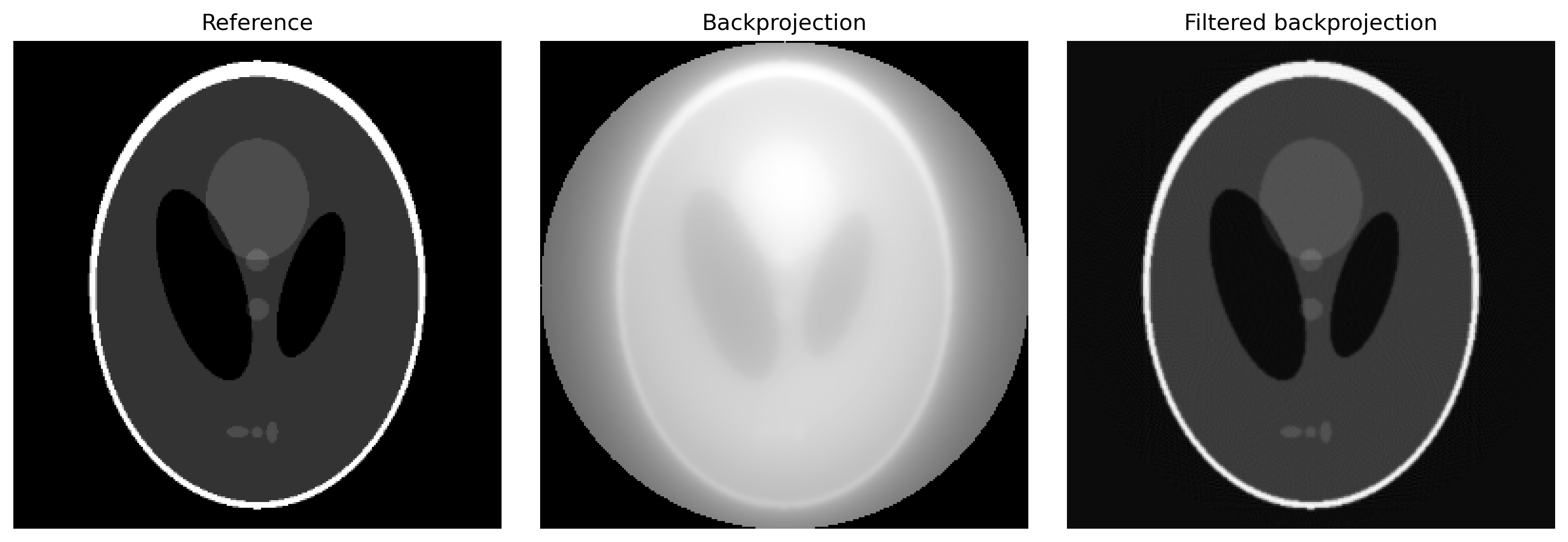
简单反投影在整个图像中形成低频拖尾;Ramp 滤波补偿频域采样密度后,边界和内部结构被恢复。这与 极坐标雅可比和 FBP 公式 的推导一致。
定量误差
代码
mse_backprojection = np.mean((image - backprojection) ** 2)
mse_fbp = np.mean((image - fbp) ** 2)

print(f"Backprojection MSE: {mse_backprojection:.6f}")
print(f"FBP MSE:            {mse_fbp:.6f}")
Backprojection MSE: 2458.159556
FBP MSE:            0.000802
库函数内部包含离散滤波、插值和尺度归一化。后续可以新增“从零实现 FBP”章节,把 FFT 频率轴、零填充、Ramp 核和角度权重逐项展开。
回到顶部